

Financial forecasting with foundation-model-based quantum reservoir computing on Cepheus-1-108Q
In a pilot with SW7 Group, FirstQFM's QRC system on Rigetti's Cepheus-1-108Q recorded the highest accuracy, macro-F1, portfolio PnL, and Sharpe ratio among the evaluated forecasting models across 43 assets and 600 out-of-sample dates.

Reservoir computing uses a high-dimensional dynamical system to transform an input sequence. It then fits a simple regularized model on the resulting features. Early work on reservoir computing used recurrent neural networks (RNNs) with randomly initialized weights as reservoirs. Time series inputs are transformed by the fixed dynamical system, yielding high-dimensional embeddings.
Quantum reservoir computing (QRC) performs that transformation with controlled quantum dynamics. For gate-based QRC, encoding operations inject the observed history, entangling gates mix information across qubits, and measured observables serve as inputs to a separate classical prediction head. This creates a feature map with temporal memory without end-to-end circuit optimization. As the number of qubits and entangling operations grows, these transformations can become exponentially more expensive to simulate classically. [1] [2]
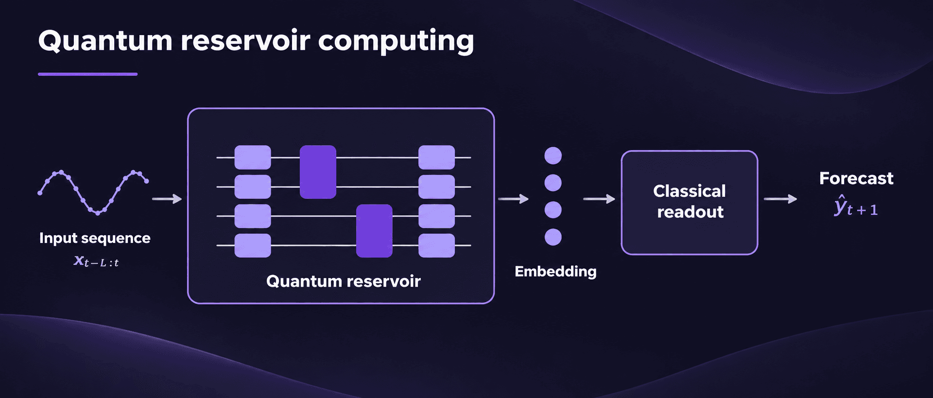
QRC can be implemented with shallow circuits and without full quantum error correction, making it suitable for implementation on noisy intermediate-scale quantum (NISQ) devices. On current processors, circuit depth, connectivity, finite-sampling error, and device noise limit what representations can be constructed. [3] [4] Furthermore, a transformation that is costly to simulate classically is not necessarily useful for forecasting.
FirstQFM extends the standard approach to QRC with a proprietary foundation model in the billion-parameter class, coupled with an end-to-end zero-shot forecasting system. The model was trained on the Leonardo supercomputer and fine-tuned on Cepheus-1-108Q. The beta system constructs problem-aware reservoirs for the forecast target and covariates, adapts them to the topology and operating conditions of the quantum processor, and applies learned stabilization to the measured quantum embeddings. [5] Its circuits balance shallow depth with the entangling structure needed for a useful feature map.
For the application in this blog post, FirstQFM deployed the beta system on Rigetti's Cepheus-1-108Q, a gate-based superconducting quantum processor built from twelve interconnected nine-qubit chiplets. [6] Every QRC forecast reported below was derived from circuits executed on Cepheus. Classical simulation was not used to generate the quantum features or forecasts.
SW7 Group supplied the task, which was to forecast the sign of the next day's return for 43 anonymized assets from 18 anonymized features. A second target recorded the return's signed magnitude, allowing forecasts to be judged by accuracy and macro-F1, as well as gross portfolio PnL and annualized Sharpe ratio. The assets, features, and calendar dates were anonymized, so the series could not be linked to external data or extended with additional observations.
| Component | Design |
|---|---|
| Forecasting problem | Next-day return direction for 43 anonymized assets |
| Information set | 18 features supplied by SW7 and observed at the forecast date with no external data |
| Out-of-sample evaluation | Six chronological test blocks, 43 assets, and 600 dates |
| Primary measures | Accuracy, macro-F1, equal-weight portfolio PnL, and annualized Sharpe ratio |
| QRC execution | FirstQFM QRC beta system on Rigetti Cepheus-1-108Q hardware |
| Comparison set | Classical statistical and machine-learning models and time series foundation models |
Among the fitted forecasting models, QRC recorded the highest observed accuracy, macro-F1, cumulative gross portfolio PnL, and Sharpe ratio, which were the targeted metrics. Its PnL was more than twice the strongest classical result, while its forecasts were the least similar to the other leading models.
Forecasting task and metrics
Each observation contained a binary target indicating the sign of the next-day asset return and a second target containing its signed magnitude. There were four primary measures of performance by which all models were evaluated:
| Measure | Interpretation |
|---|---|
| Accuracy | Share of next-period PnL directions forecast correctly |
| Macro-F1 | Average F1 score for the positive and negative classes, weighting both directions equally |
| Gross PnL | Sum of the equal-weight portfolio's realized signed outcomes over the evaluation |
| Sharpe ratio | Mean daily portfolio PnL divided by its sample standard deviation, annualized using 252 periods |
Accuracy and macro-F1 were calculated for each asset across all 600 test forecasts and then averaged equally across the 43 assets. F1 is the harmonic mean of precision and recall. Macro-F1 calculates F1 separately for each direction and averages the two scores.
For gross PnL, the forecast direction (+1 or -1) was multiplied by the corresponding realized signed return magnitude. A correct forecast earns the magnitude of the move and an incorrect forecast loses it. The 43 asset PnLs were averaged on each date, and those daily averages were summed over the 600 dates. This yields cumulative PnL without compounding.
The Sharpe ratio was calculated as the mean of that daily portfolio series divided by its sample standard deviation, multiplied by the square root of 252. It is a portfolio statistic, rather than an average of asset Sharpe ratios. Transaction costs and the risk-free rate were set to zero under the pilot definition.
Accuracy can be high when a model favors the more common direction. Macro-F1 gives both classes equal weight, while PnL captures the magnitude of correct and incorrect forecasts. Sharpe measures average portfolio PnL relative to its daily variation.
Quantum reservoir computing
A reservoir state is useful when it preserves relevant information from recent inputs while separating input histories that should lead to different predictions. In QRC, this state is accessed through measurements, rather than copied directly.
Expectation values estimated from repeated circuit execution, for example, can be used as classical features. Fujii and Nakajima introduced the modern QRC framework in “Harnessing Disordered Quantum Dynamics for Machine Learning” [1]. Their later overview [7] and the review by Mujal and colleagues [2] develop its connections to temporal information processing and near-term quantum devices.
Subsequent research has examined superconducting reservoirs and the role of noise [3], reservoir design for current quantum devices [4], and large-scale reservoir learning on analog quantum hardware [8]. Applications include food price forecasting [9], realized financial volatility [10], and multivariate time series forecasting [11].
Related work involving Rigetti has explored quantum features for recession prediction [12] and financial data streams [13]. Garvin, Kondratyev, Lipton, and Paini's "Density Matrix Classifier" [14] studies another approach to quantum feature classification.
Forecasting architecture
FirstQFM's beta QRC system offers an end-to-end forecasting pipeline, built around a quantum reservoir. For each forecast, it uses only the covariates and (optionally) target available by that date. Processing then follows four stages:
- It analyzes the target history (optionally) and aligned covariates available at the forecast date.
- It constructs a quantum reservoir suited to the problem and device conditions.
- It executes that reservoir on the quantum processor and stabilizes the resulting measurements against current hardware conditions.
- It applies a classical prediction head to return a forecast in the target's original units.
All models used the same 18 features supplied by SW7. QRC did not receive external features, asset metadata, additional observations, or a longer historical series. For this evaluation, the foundation-model weights, reservoir-generation process, embedding, and stabilization remained fixed. Device adaptation used hardware calibration and operating-condition data, not financial targets. Only the classical regression head was fitted within each fold, using its training sample and the following validation block for model selection.
Reservoir construction, data embedding, and stabilization are proprietary and protected by allowed and pending patents. Their role in the evaluation is to determine the quantum feature representation, while the separately estimated prediction head maps that representation into the units of the forecast target.
The beta model was trained for regression. For this direction forecasting task, its continuous signed-PnL forecast was converted to a class by taking its sign. Classical benchmark models included both classification models and regression models trained on signed PnL and evaluated in the same way.
The beta version of FirstQFM's model includes a pretrained head that allows zero-shot forecasting. It was excluded from this evaluation as an additional safeguard against potential data leakage. Because the asset identities and dates were anonymized, it was not possible to determine whether the unidentified underlying series appeared in the pretraining corpus of QRC or any of the time series foundation models. A new QRC head was fitted using the training observations in each fold, with settings chosen on validation data under the same chronological scheme used for the fitted benchmarks.
Training, validation, and testing
The evaluation used six consecutive 100-date test blocks. In each fold, an expanding training sample fitted the model, the next 100-observation block selected its settings, and the following 100-observation block measured performance. One unused observation separated training from validation and validation from testing.
| Test block | Training observations | Validation observations |
|---|---|---|
| 400–499 | 1–297 | 299–398 |
| 500–599 | 1–397 | 399–498 |
| 600–699 | 1–497 | 499–598 |
| 700–799 | 1–597 | 599–698 |
| 800–899 | 1–697 | 699–798 |
| 900–999 | 1–797 | 799–898 |
QRC and the classical benchmarks used the same dates, targets, embargoes, and portfolio calculations. Each fold's test observations were withheld from that fold's fitting and parameter selection. Earlier test dates could enter later training samples as time advanced. Results combine forecasts from all six test blocks into one 600-date evaluation.
Benchmark selection
Each model family used a hyperparameter search. Candidates were fitted on training data and ranked on the next validation block. Regression selection prioritized scale-normalized root mean squared error, which makes errors comparable across assets with different scales. Classification selection prioritized macro-F1.
The searches varied tree depth, leaf size, feature sampling, neural network width and depth, learning rate, component count, and regularization as appropriate to each model. For example, RF tested 12 settings with 300 trees and balanced class weights. MLP tested six combinations of hidden layers and L2 regularization (0.01 or 0.10). Histogram gradient boosting selected seven leaves, learning rate 0.05, and no L2 penalty in every fold. PLS selected one component throughout. PCR selected three components, with Ridge regularization of 10 in five folds and 1 in the remaining fold.
For random forest and multilayer perceptron (MLP) models, both regression and classification forms and alternative pooling choices were evaluated. The headline comparison reports the strongest overall construction from each family: an independently fitted random forest classifier and a pooled MLP classifier. The leading regression-to-sign models were histogram gradient boosting, partial least squares (PLS) regression, and principal-component regression with a Ridge readout.
Histogram gradient boosting adds trees sequentially to correct prediction errors and bins continuous features to make split searches efficient. PLS constructs components using their relationship with the target. Principal-component regression (PCR) instead constructs components from variation in the inputs and then uses Ridge regression to control the size of the prediction coefficients.
An individual model is fitted separately for each asset. A pooled model is fitted to observations from all 43 assets. The pooled RF and MLP used the 18 features without an asset identifier. Pooling improved MLP on all four measures. RF performed better when fitted separately by asset.
Additional models evaluated in the survey are listed in the Appendix. The results section shows the leading performers across the four targeted measures. No omitted model exceeded QRC performance on any of those measures.
Benchmark results
| Model | Forecast construction | Accuracy | Macro-F1 | PnL | Sharpe |
|---|---|---|---|---|---|
| FirstQFM QRC | Regression-to-sign | 0.5202 | 0.5176 | 513,473 | 1.22 |
| Histogram gradient boosting | Regression-to-sign | 0.5053 | 0.5028 | 91,434 | 0.58 |
| PLS regression | Regression-to-sign | 0.5062 | 0.4972 | 166,339 | 1.01 |
| PCR with Ridge | Regression-to-sign | 0.5044 | 0.4856 | 220,104 | 1.02 |
| Random forest | Classification, individual assets | 0.5066 | 0.5036 | 101,247 | 0.61 |
| MLP | Classification, pooled assets | 0.5125 | 0.5075 | 242,100 | 0.75 |
| Chronos-2 (Amazon) | Regression-to-sign, zero-shot | 0.5070 | 0.4849 | 100,071 | 0.39 |
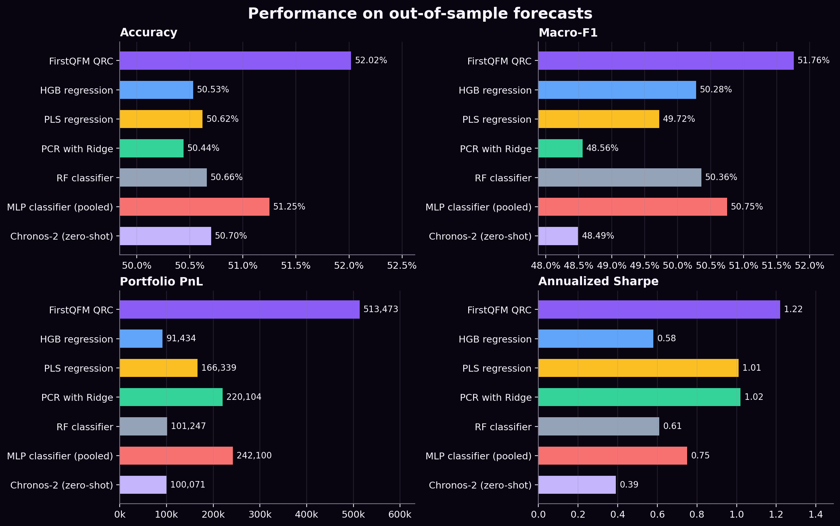
QRC achieved the best performance among the evaluated forecasting models on each targeted metric. The pooled MLP was closest on accuracy and macro-F1, with QRC ahead by 0.77 and 1.01 percentage points respectively. QRC's gross portfolio PnL was 2.12 times the pooled MLP result, the highest classical benchmark PnL. Its Sharpe of 1.22 also exceeded the strongest benchmark Sharpe ratio, which was 1.02 from PCR with Ridge.
The higher gross PnL came with greater daily PnL variation and a larger absolute drawdown. QRC's maximum peak-to-trough drawdown was 184,329, compared with 134,511 for the pooled MLP and 65,038 for PCR with Ridge. Because the models operated at different PnL scales, Sharpe provides the more comparable risk-adjusted measure.
Among the time series foundation models, zero-shot Chronos-2 had the strongest overall performance across the four targeted measures. Toto 2.0 had higher accuracy but lower macro-F1, PnL, and Sharpe. The wider exercise also evaluated task-specific Chronos-2 fine-tuning, Granite TTM-R2 (IBM) with and without adaptation, and additional foundation models that do not permit public reporting of results. No time series foundation model outperformed QRC on any targeted metrics.
While the pooled MLP and PCR models underperformed QRC across all four targeted metrics, each was profitable in 5/6 folds, compared with 4/6 for QRC.
Simple directional rules were also evaluated under the same 600-date protocol. An always-positive forecast benefited from the directional imbalance in raw accuracy but performed poorly on macro-F1 and remained below QRC on PnL and Sharpe. A direction selected from each asset's training sample produced weaker results, while one-day momentum and reversal forecasts performed close to chance and generated little financial value.
The 600-period evaluation limits the precision of the four targeted performance estimates for all models. Additionally, generalization beyond the period examined is not claimed.
Asset and portfolio results
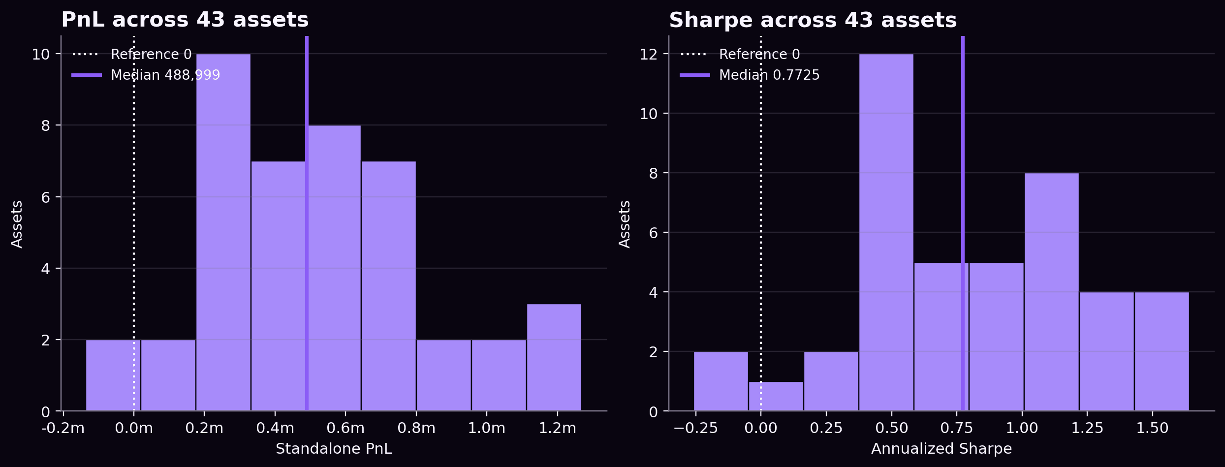
QRC achieved accuracy above 50% for 36 of 43 assets, macro-F1 above 50% for 35, and positive PnL and Sharpe for 41. For comparison, the pooled MLP produced positive PnL for 28 assets and the individual RF for 25. Median asset Sharpe was 0.77 for QRC, 0.35 for pooled MLP, and 0.10 for individual RF. QRC's financial performance extended across most of the asset universe.
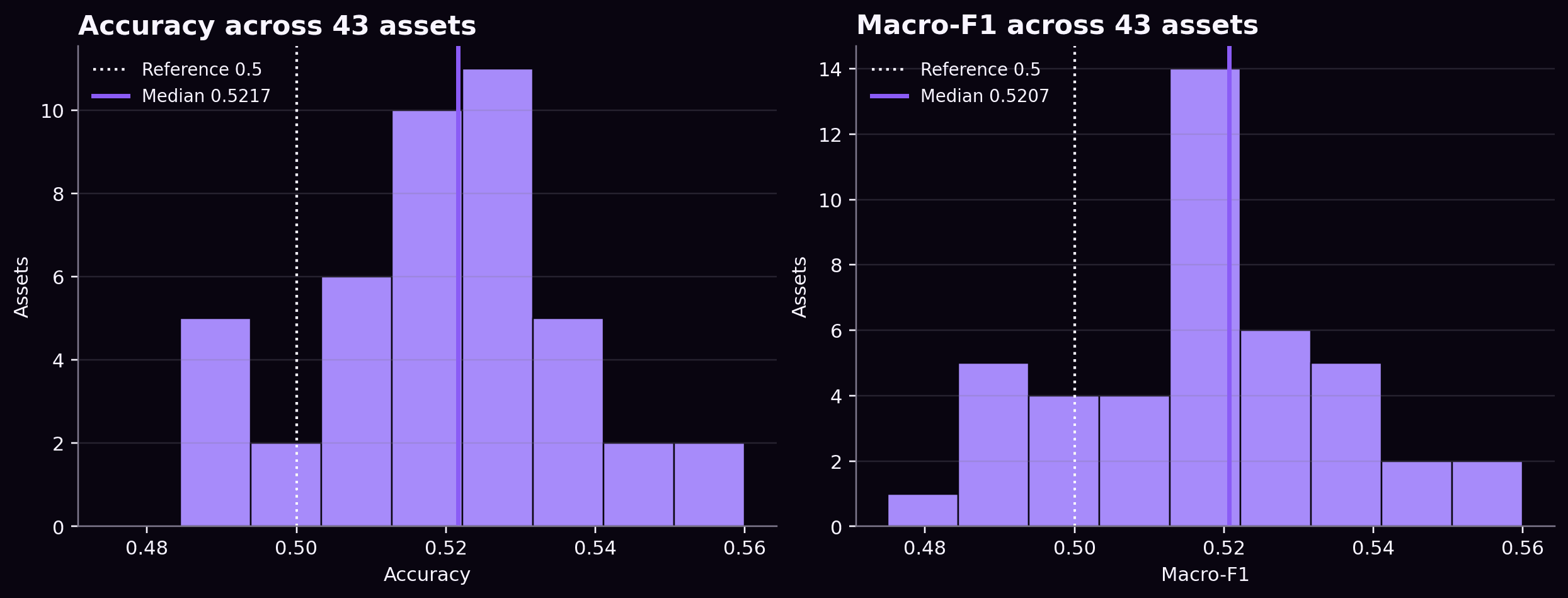
Median standalone accuracy was 52.17% and median macro-F1 was 52.07%. Median standalone PnL was 488,999 with a median Sharpe ratio of 0.77.
Portfolios of 5, 10, and 20 assets were constructed using observations 1–297. One rule ranked assets by historical model fit, measured as the share of PnL variation captured by the model. The other selected assets with low average absolute PnL correlations, adding each asset according to its correlation with those already selected. Membership stayed fixed for all 600 test dates. All six portfolios produced positive PnL, with Sharpe ratios from 0.91 to 1.73.
| Basket rule | Assets | Accuracy | Macro-F1 | PnL | Sharpe |
|---|---|---|---|---|---|
| Historical model fit | 5 | 0.5173 | 0.5166 | 484,246 | 0.91 |
| Historical model fit | 10 | 0.5212 | 0.5193 | 539,161 | 1.04 |
| Historical model fit | 20 | 0.5201 | 0.5184 | 619,369 | 1.23 |
| Historical diversification | 5 | 0.5303 | 0.5276 | 644,173 | 1.73 |
| Historical diversification | 10 | 0.5202 | 0.5160 | 464,221 | 1.24 |
| Historical diversification | 20 | 0.5210 | 0.5179 | 515,905 | 1.29 |
| All assets | 43 | 0.5202 | 0.5176 | 513,473 | 1.22 |
QRC performance for the fixed historical baskets and full equal-weight portfolio. Accuracy and macro-F1 are averages of the constituent assets' scores. PnL and Sharpe are calculated from each basket's equal-weight daily PnL series.
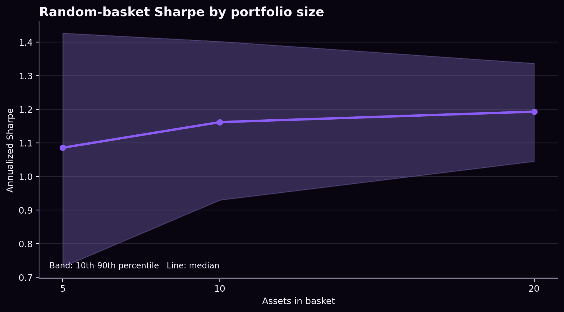
A separate sampling exercise drew 1,000 random baskets at each size. Assets were sampled uniformly without replacement within each basket, using a fixed random seed. Each basket retained its membership across all 600 dates and used the same equal-weight calculation as the full portfolio. Every sampled QRC basket produced positive cumulative PnL.
Forecast differences
For each pair of models, disagreement is the fraction of asset forecasts for which they predict opposite directions. Averaging this fraction across the other five models gives each model's value in Figure 6. QRC had the highest average disagreement at 49.0%, followed by pooled MLP at 46.8%.
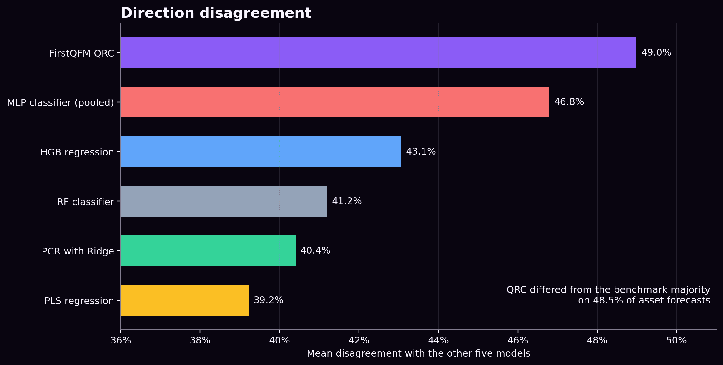
The benchmark consensus was the direction predicted by at least three of the five classical benchmark models. QRC opposed it on 48.5% of all asset forecasts. On those observations, QRC was correct 50.89% of the time and the majority was correct 49.11% of the time. QRC's mean PnL exceeded the majority forecast by 971 per asset observation.
QRC combined stronger aggregate results with predictions that often differed from the benchmarks. This suggests that the QRC model could be a strong contributor to an ensemble.
Quantum hardware
All reported QRC outputs were generated on Rigetti's Cepheus-1-108Q quantum processor. The evaluation used 600 forecast-date reservoir evaluations ranging from 61 to 84 physical qubits. Each evaluation contributed to the system's forecasts for all 43 assets on that date.
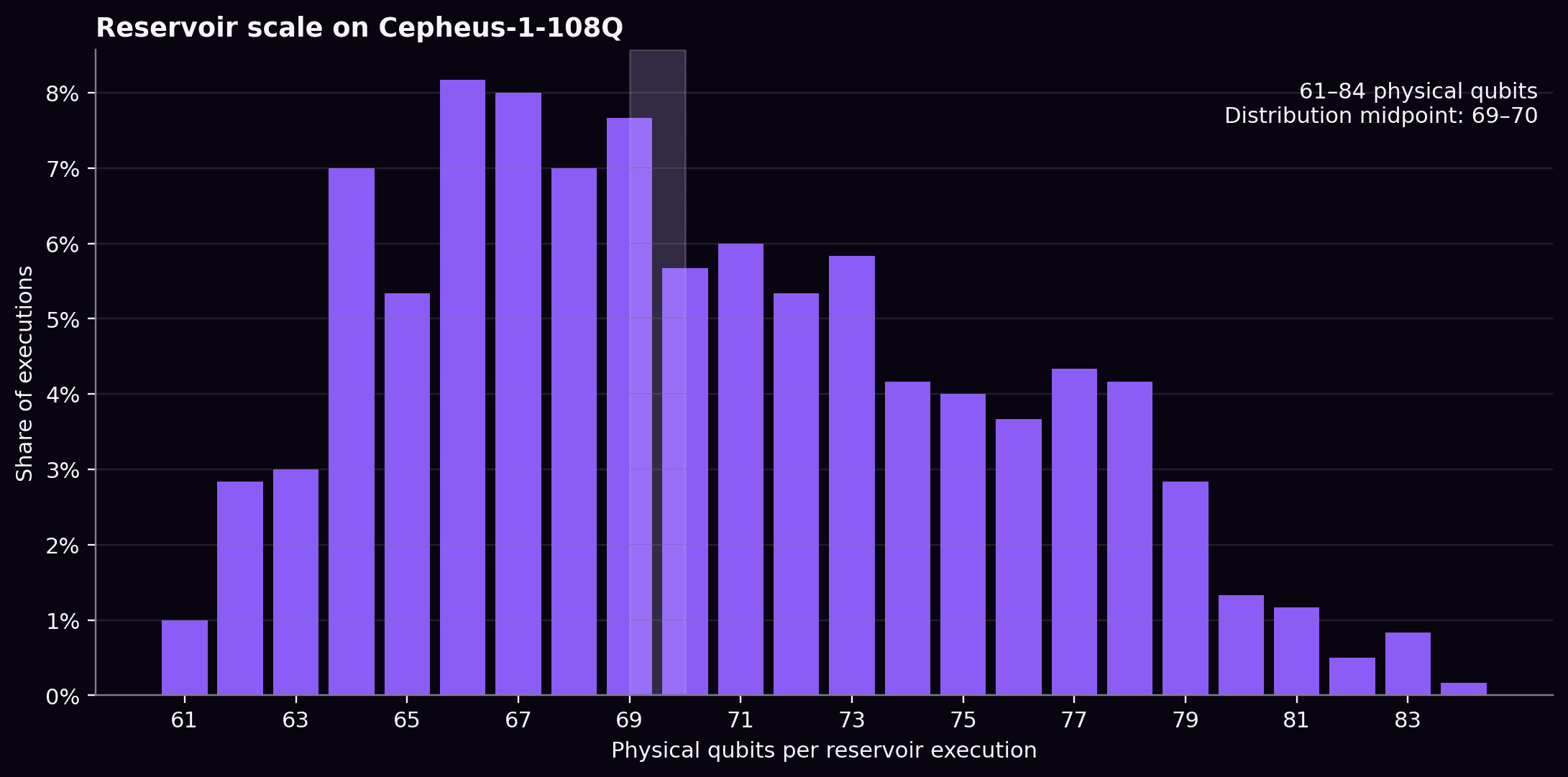
Reservoir construction accounts for device connectivity and noise. The circuits balance a depth suitable for the hardware with enough entangling operations to support useful reservoir dynamics. Stabilization converts measurements obtained under changing hardware conditions into consistent inputs for the prediction head.
The number of qubits and number of entangling operations makes classical simulation non-trivial, but no formal claim of non-simulability is made, as this is a moving target that depends on evolving classical methods.
Conclusion
FirstQFM's QRC system achieved the highest observed accuracy, macro-F1, gross portfolio PnL, and annualized Sharpe ratio among the fitted forecasting models in aggregate results across 43 assets and 600 forecast periods. It produced positive PnL for 41 of 43 assets and frequently disagreed with the benchmark consensus. These results were based on measurements on Rigetti's Cepheus-1-108Q with prediction heads fitted and validated chronologically on SW7's data.
QRC and all fitted classical benchmarks used the same supplied features, dates, targets, chronological training, validation, and test folds, and evaluation formulas. The zero-shot time series foundation models were pretrained and therefore were not fitted on the pilot training folds. Their adapted variants, where reported, used the pilot's chronological folds.
Cepheus-1-108Q combines the size and performance needed to execute the pilot's 61 to 84-qubit reservoirs, along with fast-executing superconducting gates, which support the repeated circuit executions needed for QRC. This makes it an especially promising platform for latency-sensitive QRC applications.
No broader form of "quantum advantage" or generalization of performance beyond the models and periods evaluated is claimed.
References
- K. Fujii and K. Nakajima, “Harnessing Disordered Quantum Dynamics for Machine Learning”, Physical Review Applied 8, 024030, 2017.
- P. Mujal et al., “Opportunities in Quantum Reservoir Computing and Extreme Learning Machines”, Advanced Quantum Technologies 4, 2100027, 2021.
- Y. Suzuki et al., “Natural Quantum Reservoir Computing for Temporal Information Processing”, Scientific Reports 12, 1353, 2022.
- L. Domingo, G. Carlo, and F. Borondo, “Optimal Quantum Reservoir Computing for the NISQ Era”, Physical Review E 106, L043301, 2022.
- FirstQFM, “Foundation-Model QRC for Enterprise Forecasting”, 2026.
- Rigetti Computing, “Rigetti Announces General Availability of 108-Qubit System”, 2026.
- K. Fujii and K. Nakajima, “Quantum Reservoir Computing: A Reservoir Approach Toward Quantum Machine Learning on Near-Term Quantum Devices”, 2021.
- M. Kornjača et al., “Large-Scale Quantum Reservoir Learning with an Analog Quantum Computer”, 2024.
- L. Domingo et al., “Optimal Quantum Reservoir Computing for Market Forecasting: An Application to Fight Food Price Crises”, 2024.
- Q. Li et al., “Quantum Reservoir Computing for Realized Volatility Forecasting”, 2025.
- W. Hamhoum et al., “Multivariate Time Series Forecasting with Gate-Based Quantum Reservoir Computing on NISQ Hardware”, 2025.
- Rigetti Computing, Moody's Analytics, and Imperial College London, “Recession Prediction via Signature Kernels Enhanced with Quantum Features”, 2023.
- Rigetti Computing, Imperial College London, Standard Chartered, National Tsing Hua University, and Amazon Web Services, “Exact Simulation of Quantum Enhanced Signature Kernels for Financial Data Streams Prediction Using Amazon Braket”, 2025.
- D. Garvin, O. Kondratyev, A. Lipton, and M. Paini, “Density Matrix Classifier”, SSRN working paper, 2024.
Appendix
| Comparison family | Additional models and constructions evaluated |
|---|---|
| Linear and robust regression | Ridge, Huber, elastic net, and pooled elastic net |
| Support vector models | Linear and radial-basis support vector classification, and radial-basis support vector regression |
| Classification and discriminant models | Logistic and pooled logistic regression, shrinkage linear discriminant analysis, and regularized quadratic discriminant analysis |
| Trees and boosting | Random forest regression, pooled random forest classification, Extra Trees classification and regression, histogram gradient boosting classification, and XGBoost classification and regression in individual and pooled forms |
| Neural models | Individual MLP classification, MLP regression, and classification and regression ensembles |
| Reservoir computing models | Echo state network, random Fourier feature model, dense random nonlinear map |
| Time series foundation models | Fine-tuned Chronos-2 (Amazon), zero-shot and adapted Granite TTM-R2 (IBM), Toto 2.0 (Datadog), and additional internally evaluated models with licenses that do not permit a public comparison of results. |
Keep reading
Foundation model-based QRC for enterprise time series forecasting
FirstQFM's alpha-version system outperformed leading time series foundation model baselines on selected zero shot forecasting tasks across held-out series. We are now announcing a broader beta system release to pilot partners.

Is quantum computing’s future in the hands of AI?
A perspective on AI-guided quantum technology, and what “quantum advantage” means.